Georeferencing PennPilot aerial imagery
This video covers my approach to georeferencing old aerial photos as I work on a series of Horse-Shoe Trail Maps (a personal project). Key points include using a similar period USGS Quad as a reference, using the index to select an aerial for an area, and cropping the images.
Georeferencing, aka rubbersheeting, requires patience. I’m going to go over the process I am using to align photos for the Horse-Shoe Trail maps I’m working on. I’ll be doing this in QGIS.
Data sources
I used black and white PennPilot aerial photos from 1937-1942. These are now hosted at pasda.psu.edu. I downloaded directories for the years and counties I needed using an ftp program (Transmit). Each directory has a couple of index files as well as maps at different resolutions. I used the tifs instead of the highest resolution jpgs, but I don’t think it matters.
Selecting aerials
I created a buffer around the map panels and then selected index points that fell within the buffer. This wasn’t necessary, but it gave me a sense for how many aerial images I’d end up working with.
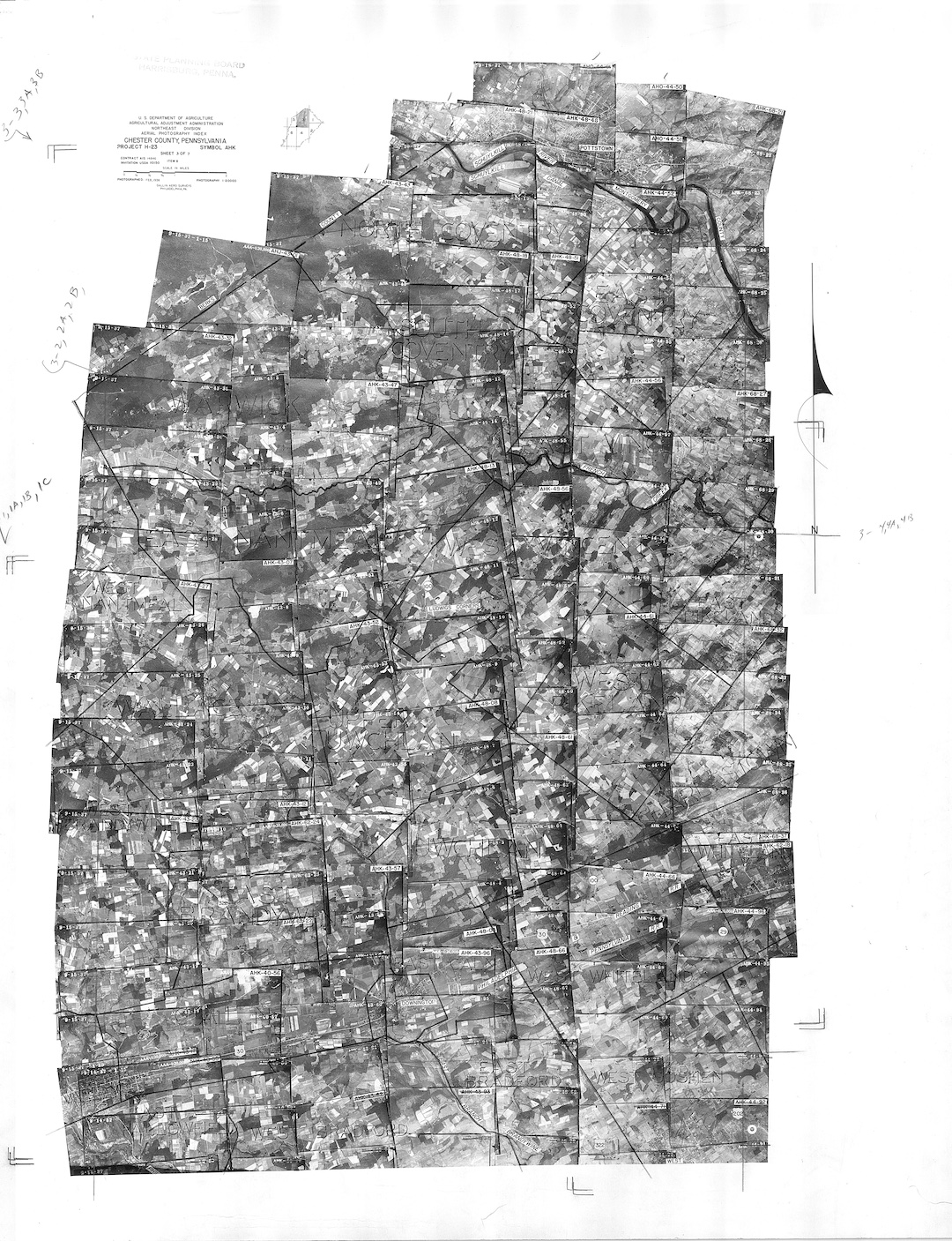
There’s a shapefile index called something like “Chester_1937_photocorners” that shows the approximate Northeast corner of each image. There’s also a georeferenced image of overlapping images. I printed the image out to use as a reference.
Here’s what an associated PennPilot geotif index looks like:
Base image or map to reference against
I initially used google aerial imagery. But the landscape had changed so much that I decided to use topographic maps closer to the 1930’s. This made finding matching features easier. The topographic quadrangles came from https://ngmdb.usgs.gov/topoview/viewer/#4/40.00/-100.00.
Regardless of the base, it needs to be loaded in the projection you want. I used web mercator.
Adding (geoprocessing coordinates)
In the QGIS raster menu, there’s an option for georeferencing. Select an image to georeference. Then you find matching points between the image and the currently projected reference map. Zoom in to as large of a scale as possible for better accuracy.
Place points throughout the image. You’ll need a minimum of 6 points, but 10 or more is helpful, making sure there are plenty of points near the perimeter of the image.
If points really seem misaligned, you’ll see a line to a point that shows the problem spot.
Transforming the image
There’s a “play” button that places a version of the image over the base map. You’ll get a dialog asking you to name the georeferenced image, but I just use the default and then hit the play button again.
If things don’t line up perfectly, which they won’t, you can delete or move problem points and add new points.
Unwanted black boundaries
The resulting georeferenced images will likely have black boundaries. I was able to remove these by setting the minimum value to 1. This removed black areas within the image, so I resent the minimum value of the image to 0 and decided to go with a cropping approach.
To crop, I drew a temporary polygon over each aerial to clip the black area off of the raster image.
When doing this, I still got a black area surrounding the image. To avoid this, I checked the following options:
- Create an alpha layer
- Match the extent of the clipped raster to the output band
- Keep resolution of input raster
Tiling the maps
I merged the cropped imagery into a single image by map only to see imperfections in the results.
Summary
Georeferencing the first map took me a long time (a couple of days). I was trying to figure out a fast way to do it. I wondered if I should compare photo to photo or if I should compare photo to google satellite imagery. And I wondered if it was even worth doing. Importing USGS topos helped.
Students at Penn State were discussing using algorithms to match up aerials. It’s obvious to me why nobody has georeferenced the old maps on a county by county scale. Well, Center County is done, and one can still see misalignments. But I bet this was done as part of an exercise in learning to georeference imagery.
I spent a lot of time looking at the images in detail that I felt like I gained a historical perspective. In 1937 there might have been a newly planted orchard. And there may have been a dam in the Schuylkill River. I saw a lot of quarries. So, through this effort, I learned.
Future work
I expect it will take a full month to georeference all twenty maps because a single map panel in my book can involve 8 aerials. Once done, they may not be all that useful at 1:39,000 scale. I might try to colorize one or two to see what I can learn.
The densities of grays from photo to photo don’t match. I may look into fixing this.